The typical database contains many tables. Some smaller databases may have only a dozen or so tables, whereas other databases may have hundreds or even thousands. The common factor, however, is that few databases have just one table containing everything you need. Therefore, you usually have to draw data from multiple tables together in a meaningful way. To show data from multiple tables in one query, Oracle allows you to perform table joins.
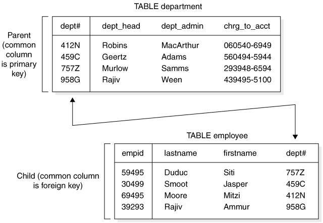
Here are the two rules you need to remember for table joins. Data from two (or more) tables can be joined, if the same column (under the same or a different name) appears in both tables, and the column is the primary key (or part of that key) in one of the tables. Having a common column in two tables implies a relationship between the two tables. The nature of that relationship is determined by which table uses the column as a primary key. This begs the question, what is a primary key? A primary key is a column in a table used for identifying the uniqueness of each row in a table. The table in which the column appears as a primary key is referred to as the parent table in this relationship (sometimes also called the master table), whereas the column that references the other table in the relationship is often called the child table (sometimes also called the detail table). The common column appearing in the child table is referred to as a foreign key.

Join Syntax
Let’s look at an example of a join statement using the Oracle traditional syntax, where we join the contents of the EMP and DEPT tables together to obtain a listing of all employees, along with the names of the departments they work for:

SQL> select e.ename, e.deptno, d.dname
    2  from emp e, dept d
    3  where e.deptno = d.deptno;

ENAME     DEPTNO    DNAME
———-      ———     ————–
SMITH         20          RESEARCH
ALLEN         30          SALES
WARD         30          SALES
JONES         20          RESEARCH
Note the many important components in this table join. Listing two tables in the from clause clearly indicates that a table join is taking place. Note also that each table name is followed by a letter: E for EMP or D for DEPT. This demonstrates an interesting concept—just as columns can have aliases, so too can tables. The aliases serve an important purpose—they prevent Oracle from getting confused about which table to use when listing the data in the DEPTNO column. Remember, EMP and DEPT both have a column named DEPTNO
You can also avoid ambiguity in table joins by prefixing references to the columns with the table names, but this often requires extra coding. You can also give the column two different names, but then you might forget that the relationship exists between the two tables. It’s just better to use aliases! Notice something else, though. Neither the alias nor the full table name needs to be specified for columns appearing in only one table. Take a look at another example:
SQL> select ename, emp.deptno, dname
  2  from emp, dept
  3  where emp.deptno = dept.deptno;
How Many Comparisons Do You Need?
When using Oracle syntax for table joins, a query on data from more than two tables must contain the right number of equality operations to avoid a Cartesian product. To avoid confusion, use this simple rule: If the number of tables to be joined equals N, include at least N-1 equality conditions in the select statement so that each common column is referenced at least once. Similarly, if you are using the ANSI/ISO syntax for table joins, you need to use N-1 join tablename on join_condition clauses for every N tables being joined.

For N joined tables using Oracle or ANSI/ISO syntax for table joins, you need at least N-1 equijoin conditions in the where clause of your select statement or N-1 join tablename on join_condition clauses in order to avoid a Cartesian product, respectively.

Cartesian Products
Notice also that our where clause includes a comparison on DEPTNO linking data in EMP to that of DEPT. Without this link, the output would have included all data from EMP and DEPT, jumbled together in a mess called a Cartesian product. Cartesian products are big, meaningless listings of output that are nearly never what you want. They are formed when you omit a join condition in your SQL statement, which causes Oracle to join all rows in the first table to all rows in the second table. Let’s look at a simple example in which we attempt to join two tables, each with three rows, using a select statement with no where clause, resulting in output with nine rows:

SQL> select a.col1, b.col_2
  2  from example_1 a, example_2 b;

     COL1 COL_2
——— ——————————
        1 one
        2 one
        3 one
        1 two
        2 two
        3 two
You must always remember to include join conditions in join queries to avoid Cartesian products. But take note of another important fact. Although we know that where clauses can contain comparison operations other than equality, to avoid Cartesian products, you must always use equality operations in a comparison joining data from two tables. If you want to use another comparison operation, you must first join the information using an equality comparison and then perform the other comparison somewhere else in the where clause. This is why table join operations are also sometimes referred to as equijoins. Take a look at the following example that shows proper construction of a table join, where the information being joined is compared further using a nonequality operation to eliminate the employees from accounting:

SQL> select ename, emp.deptno, dname
  2  from emp, dept
  3  where emp.deptno = dept.deptno
  4  and dept.deptno > 10;

ANSI/ISO Join Syntax (Oracle9i and higher)
In Oracle9i, Oracle introduces strengthened support for ANSI/ISO join syntax. To join the contents of two tables together in a single result according to that syntax, we must include a join tablename on join_condition in our SQL statement. If we wanted to perform the same table join as before using this new syntax, our SQL statement would look like the following:
Select ename, emp.deptno, dname
from emp join dept
on emp.deptno = dept.deptno;

ENAME         DEPTNO    DNAME
———-          ———      ————–
SMITH             20         RESEARCH
ALLEN             30         SALES
WARD             30         SALES
JONES             20         RESEARCH

Note how different this is from Oracle syntax. First, ANSI/ISO syntax separates join comparisons from all other comparisons by using a special keyword, on, to indicate what the join comparison is. You can still include a where clause in your ANSI/ISO-compliant join query, the only difference is that the where clause will contain only those additional conditions you want to use for filtering your data. You also do not list all your tables being queried in one from clause. Instead, you use the join clause directly after the from clause to identify the table being joined.
Never combine Oracle’s join syntax with ANSI/ISO’s join syntax! Also, there are no performance differences between Oracle join syntax and ANSI/ISO join syntax.
Cartesian Products: An ANSI/ISO Perspective
In some cases, you might actually want to retrieve a Cartesian product, particularly in financial applications where you have a table of numbers that needs to be cross-multiplied with another table of numbers for statistical analysis purposes. ANSI/ISO makes a provision in its syntax for producing Cartesian products through the use of a cross-join. A cross-join is produced when you use the cross keyword in your ANSI/ISO-compliant join query. Recall from a previous example that we produced a Cartesian product by omitting the where clause when joining two sample tables, each containing three rows, to produce nine rows of output. We can produce this same result in ANSI/ISO SQL by using the cross keyword, as shown here in bold:

Select col1, col_2
from example_1 cross join example_2;

COL1    COL_2
——— ————-
 1        one
 2        one
 3        one
 1        two
 2        two
 3        two
 1        three

Natural Joins

One additional type of join you need to know about for OCP is the natural join. A natural join is a join between two tables where Oracle joins the tables according to the column(s) in the two tables sharing the same name (naturally!). Natural joins are executed whenever the natural keyword is present. Let’s look at an example. Recall our use of the EMP and DEPT tables from our discussion above. Let’s take a quick look at the column listings for both tables:
SQL> describe emp
Name                       Null            Type
————————–    ———       ————
EMPNO                  NOT NULL    NUMBER(4)
ENAME                                    VARCHAR2(10)
JOB                                         VARCHAR2(9)
MGR                                        NUMBER(4)
SQL> describe dept
Name                       Null           Type
————————–   ———       ————
DEPTNO                 NOT NULL  NUMBER(2)
DNAME                                   VARCHAR2(14)
LOC                                       VARCHAR2(13)
As you can see, DEPTNO is the only column in common between these two tables, and appropriately enough, it has the same name in both tables. This combination of facts makes our join query of EMP and DEPT tables a perfect candidate for a natural join. Take a look and see:
Select ename, deptno, dname
from emp natural join dept;

ENAME         DEPTNO    DNAME
———-          ———    ————–
SMITH             20         RESEARCH
ALLEN             30         SALES
WARD             30         SALES
Outer Joins
Outer joins extend the capacity of Oracle queries to include handling of situations where you want to see information from tables even when no corresponding records exist in the common column.  The purpose of an outer join is to include non-matching rows, and the outer join returns these missing columns as NULL values.
Left Outer Join
A left outer join will return all the rows that an inner join returns plus one row for each of the other rows in the first table that did not have a match in the second table.
Suppose you want to find all employees and the projects they are currently responsible for. You want to see those employees that are not currently in charge of a project as well. The following query will return a list of all employees whose names are greater than ‘S’, along with their assigned project numbers.
  SELECT EMPNO, LASTNAME, PROJNO
    FROM CORPDATA.EMPLOYEE LEFT OUTER JOIN CORPDATA.PROJECT
          ON EMPNO = RESPEMP
    WHERE LASTNAME > ‘S’
The result of this query contains some employees that do not have a project number. They are listed in the query, but have the null value returned for their project number.
EMPNO     LASTNAME     PROJNO
000020     THOMPSON     PL2100
000100     SPENSER         OP2010
000170     YOSHIMURA     –
000250     SMITH             AD3112
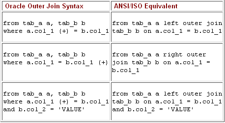
In oracle we can specify(in Oracle 8i or prior vesrion this was the only option as they were not supporting the ANSI syntex) left outer join by putting a (+) sign on the right of the column which can have NULL data corresponding to non-NULL values in the column values from the other table.
example:  select    last_name,   department_name
from   employees e,   departments d
where  
e.department_id(+) = d.department_id;
Right Outer Join
A right outer join will return all the rows that an inner join returns plus one row for each of the other rows in the second table that did not have a match in the first table. It is the same as a left outer join with the tables specified in the opposite order.
The query that was used as the left outer join example could be rewritten as a right outer join as follows:

SQL> — Earlier version of outer join
SQL> — select e.ename, e.deptno, d.dname
SQL> — from dept d, emp e
SQL> — where d.deptno = e.deptno (+);
SQL>
SQL> — ANSI/ISO version
SQL> select e.ename, e.deptno, d.dname
SQL> from emp e right outer join dept d
SQL> on d.deptno = e.deptno;

Full Outer Joins
Oracle9i and higher
Oracle9i also makes it possible for you to easily execute a full outer join, including all records from the tables that would have been displayed if you had used both the left outer join or right outer join clauses. Let’s take a look at an example:
SQL> select e.ename, e.deptno, d.dname
2 from emp e full outer join dept d
3 on d.deptno = e.deptno;

So far, we have seen how to get data out of a table using SELECT and WHERE commands. Often, however, we need to list the output in a particular order. This could be in ascending order, in descending order, or could be based on either numerical value or text value. In such cases, we can use the ORDER BY keyword to achieve our goal.
The syntax for an ORDER BY statement is as follows:

SELECT “column_name”
FROM “table_name”
[WHERE “condition”]
ORDER BY “column_name” [ASC, DESC]

The [] means that the WHERE statement is optional. However, if a WHERE clause exists, it comes before the ORDER BY clause. ASC means that the results will be shown in ascending order, and DESC means that the results will be shown in descending order. If neither is specified, the default is ASC.
It is possible to order by more than one column. In this case, the ORDER BY clause above becomes ORDER BY “column_name1” [ASC, DESC], “column_name2” [ASC, DESC]
 The SQL HAVING clause is used to restrict conditionally the output of a SQL statement, by a SQL aggregate function used in your SELECT list of columns.
SELECT column1, column2, … column_n, aggregate_function (expression)
FROM tables
WHERE predicates
GROUP BY column1, column2, … column_n
HAVING condition1 … condition_n;

You can’t specify criteria in a SQL WHERE clause against a column in the SELECT list for which SQL aggregate function is used. For example the following SQL statement will generate an error:
SELECT Employee, SUM (Hours)
FROM EmployeeHours
WHERE SUM (Hours) > 24
GROUP BY Employee
The SQL HAVING clause is used to do exactly this, to specify a condition for an aggregate function which is used in your query:
SELECT Employee, SUM (Hours)
FROM EmployeeHours
GROUP BY Employee
HAVING SUM (Hours) > 24
Group functions allow you to perform data operations on several values in a column of data as though the column were one collective group of data. These functions are also called group-by functions because they are often used in a special clause of select statements, called the group by clause.
The syntax for the GROUP BY clause is:
    SELECT column1, column2, … column_n, aggregate_function (expression)
    FROM tables
    WHERE predicates
    GROUP BY column1, column2, … column_n;
aggregate_function can be a function such as SUM, COUNT, MIN, or MAX.
Here’s a list of the available group functions:

  • avg(x) Averages all x column values returned by the select statement
  • count(x) Counts the number of non-NULL values returned by the select statement for column x
  • max(x) Determines the maximum value in column x for all rows returned by the select statement
  • min(x) Determines the minimum value in column x for all rows returned by the select statement
  • stddev(x) Calculates the standard deviation for all values in column x in all rows returned by the select statement
  • sum(x) Calculates the sum of all values in column x in all rows returned by the select statement
  • Variance(x) Calculates the variance for all values in column x in all rows returned by the select statement

Example using the SUM function
For example, you could also use the SUM function to return the name of the department and the total sales (in the associated department).
SELECT department, SUM(sales) as “Total sales”
FROM order_details
GROUP BY department;

Because you have listed one column in your SELECT statement that is not encapsulated in the SUM function, you must use a GROUP BY clause. The department field must, therefore, be listed in the GROUP BY section.
Example using the COUNT function
For example, you could use the COUNT function to return the name of the department and the number of employees (in the associated department) that make over $25,000 / year.
SELECT department, COUNT(*) as “Number of employees”
FROM employees
WHERE salary > 25000
GROUP BY department;
ROLLUP
This group by operation is used to produce subtotals at any level of aggregation needed. These subtotals then “roll up” into a grand total, according to items listed in the group by expression. The totaling is based on a one-dimensional data hierarchy of grouped information. For example, let’s say we wanted to get a payroll breakdown for our company by department and job position. The following code block would give us that information:
SQL> select deptno, job, sum(sal) as salary
  2  from emp
  3  group by rollup(deptno, job);
   DEPTNO JOB          SALARY
——— ——— ———
       10 CLERK          1300
       10 MANAGER        2450
       10 PRESIDENT      5000
       10                8750
       20 ANALYST        6000
       20 CLERK          1900
       20 MANAGER        2975
       20               10875
       30 CLERK           950
       30 MANAGER        2850
       30 SALESMAN       5600
       30                9400
                        29025
Notice that NULL values in the output of rollup operations typically mean that the row contains subtotal or grand total information. If you want, you can use the nvl( ) function to substitute a more meaningful value.
cube
cube This is an extension, similar to rollup. The difference is that cube allows you to take a specified set of grouping columns and create subtotals for all possible combinations of them. The cube operation calculates all levels of subtotals on horizontal lines across spreadsheets of output and creates cross-tab summaries on multiple vertical columns in those spreadsheets. The result is a summary that shows subtotals for every combination of columns or expressions in the group by clause, which is also known as n-dimensional cross-tabulation. In the following example, notice how cube not only gives us the payroll breakdown of our company by DEPTNO and JOB, but it also gives us the breakdown of payroll by JOB across all departments:
SQL>  select deptno, job, sum(sal) as salary
  2  from emp
  3  group by cube(deptno, job);
DEPTNO JOB          SALARY
——— ——— ———
       10 CLERK          1300
       10 MANAGER        2450
       10 PRESIDENT      5000
       10                8750
       20 ANALYST        6000
       20 CLERK          1900
       20 MANAGER        2975
       20               10875
       30 CLERK           950
       30 MANAGER        2850
       30 SALESMAN       5600
       30                9400
          ANALYST        6000
          CLERK          4150
          MANAGER        8275
          PRESIDENT      5000
          SALESMAN       5600
                        29025
Excluding group Data with having
Once the data is grouped using the group by statement, it is sometimes useful to weed out unwanted data. For example, let’s say we want to list the average salary paid to employees in our company, broken down by department and job title. However, for this query, we only care about departments and job titles where the average salary is over $2000. In effect, we want to put a where clause on the group by clause to limit the results we see to departments and job titles where the average salary equals $2001 or higher. This effect can be achieved with the use of a special clause called the having clause, which is associated with group by statements. Take a look at an example of this clause:
SQL> select deptno, job, avg(sal)
  2  from emp
  3  group by deptno, job
  4  having avg(sal) > 2000;
   DEPTNO JOB        AVG(SAL)
———     ———           ———
       10   MANAGER        2450
       10   PRESIDENT      5000
       20   ANALYST        3000
       20   MANAGER        2975
       30   MANAGER        2850
Consider the output of this query for a moment. First, Oracle computes the average for every department and job title in the entire company. Then, the having clause eliminates departments and titles whose constituent employees’ average salary is $2000 or less. This selectivity cannot easily be accomplished with an ordinary where clause, because the where clause selects individual rows, whereas this example requires that groups of rows be selected. In this query, you successfully limit output on the group by rows by using the having clause.

The SQL WHERE clause is used to select data conditionally, by adding it to already existing SQL SELECT query. We are going to use the Customers table from the previous chapter, to illustrate the use of the SQL WHERE command.
Syntax
SELECT column_name(s)
FROM table_name
WHERE column_name operator value

With the WHERE clause, the following operators can be used:
Operator     Description
=     Equal
<>     Not equal
>     Greater than
<     Less than
>=     Greater than or equal
<=     Less than or equal
LIKE     Search for a pattern
IN     If you know the exact value you want to return for at least one of the columns
BETWEEN     Between an inclusive range
“AND” Condition
The AND condition allows you to create an SQL statement based on 2 or more conditions being met. It can be used in any valid SQL statement – select, insert, update, or delete.
The syntax for the AND condition is:
    SELECT columns
    FROM tables
    WHERE column1 = ‘value1’
    and column2 = ‘value2’;

The AND condition requires that each condition be must be met for the record to be included in the result set. In this case, column1 has to equal ‘value1’ and column2 has to equal ‘value2’.
“OR” Condition
The OR condition allows you to create an SQL statement where records are returned when any one of the conditions are met. It can be used in any valid SQL statement – select, insert, update, or delete.
The syntax for the OR condition is:
    SELECT columns
    FROM tables
    WHERE column1 = ‘value1’
    or column2 = ‘value2’;
The OR condition requires that any of the conditions be must be met for the record to be included in the result set. In this case, column1 has to equal ‘value1’ OR column2 has to equal ‘value2’.
Combining the “AND” and “OR” Conditions
The AND and OR conditions can be combined in a single SQL statement. It can be used in any valid SQL statement – select, insert, update, or delete. When combining these conditions, it is important to use brackets so that the database knows what order to evaluate each condition.
Example
The first example that we’ll take a look at an example that combines the AND and OR conditions.
    SELECT *
    FROM suppliers
    WHERE (city = ‘New York’ and name = ‘IBM’)
    or (city = ‘Newark’);
LIKE Operator
The LIKE operator is used to search for a specified pattern in a column.
SQL LIKE Syntax
SELECT column_name(s)
FROM table_name
WHERE column_name LIKE pattern
The LIKE condition can be used in any valid SQL statement – select, insert, update, or delete.
The patterns that you can choose from are:
    % allows you to match any string of any length (including zero length)
    _ allows you to match on a single character

Examples using % wildcard
The first example that we’ll take a look at involves using % in the where clause of a select statement. We are going to try to find all of the suppliers whose name begins with ‘Hew’.
SELECT *
FROM suppliers
WHERE supplier_name like ‘Hew%’;
You can also using the wildcard multiple times within the same string. For example,
SELECT *
FROM suppliers
WHERE supplier_name like ‘%bob%’;
Examples using _ wildcard
Next, let’s explain how the _ wildcard works. Remember that the _ is looking for only one character.
For example,
SELECT *
FROM suppliers
WHERE supplier_name like ‘Sm_th’;
This SQL statement would return all suppliers whose name is 5 characters long, where the first two characters is ‘Sm’ and the last two characters is ‘th’. For example, it could return suppliers whose name is ‘Smith’, ‘Smyth’, ‘Smath’, ‘Smeth’, etc.
IN Function
The IN operator allows you to specify multiple values in a WHERE clause.
SELECT column_name(s)
FROM table_name
WHERE column_name IN (value1,value2,…)

The following is an SQL statement that uses the IN function:
SELECT *
FROM suppliers
WHERE supplier_name in ( ‘IBM’, ‘Hewlett Packard’, ‘Microsoft’);
This would return all rows where the supplier_name is either IBM, Hewlett Packard, or Microsoft. Because the * is used in the select, all fields from the suppliers table would appear in the result set.
It is equivalent to the following statement:
SELECT *
FROM suppliers
WHERE supplier_name = ‘IBM’
OR supplier_name = ‘Hewlett Packard’
OR supplier_name = ‘Microsoft’;
As you can see, using the IN function makes the statement easier to read and more efficient.
BETWEEN
The BETWEEN condition allows you to retrieve values within a range.
The syntax for the BETWEEN condition is:
SELECT columns
FROM tables
WHERE column1 between value1 and value2;

This SQL statement will return the records where column1 is within the range of value1 and value2 (inclusive). The BETWEEN function can be used in any valid SQL statement – select, insert, update, or delete.
The following is an SQL statement that uses the BETWEEN function:
SELECT *
FROM suppliers
WHERE supplier_id between 5000 AND 5010;
This would return all rows where the supplier_id is between 5000 and 5010, inclusive. It is equivalent to the following SQL statement:
SELECT *
FROM suppliers
WHERE supplier_id >= 5000
AND supplier_id <= 5010;
EXISTS Condition
The EXISTS condition is considered “to be met” if the subquery returns at least one row.
The syntax for the EXISTS condition is:
SELECT columns
FROM tables
WHERE EXISTS ( subquery );

The EXISTS condition can be used in any valid SQL statement – select, insert, update, or delete.
Example1:
Let’s take a look at a simple example. The following is an SQL statement that uses the EXISTS condition:
SELECT *
FROM suppliers
WHERE EXISTS (select *  from orders where suppliers.supplier_id = orders.supplier_id);
This select statement will return all records from the suppliers table where there is at least one record in the orders table with the same supplier_id.
Example 2: NOT EXISTS
The EXISTS condition can also be combined with the NOT operator.
For example,
SELECT *    FROM suppliers  WHERE not exists (select * from orders Where suppliers.supplier_id = orders.supplier_id);
This will return all records from the suppliers table where there are no records in the orders table for the given supplier_id.
Example 3:  DELETE Statement
The following is an example of a delete statement that utilizes the EXISTS condition:
DELETE FROM suppliers  WHERE EXISTS (select * from orders where suppliers.supplier_id = orders.supplier_id);